This function checks the proportional hazards assumption in the Cox model using Schoenfeld residuals. This function only return results for strategies based on efficient influence functions.
Usage
# S3 method for class 'tteICE'
zph(x)Value
A list of P-values of testing the proportional hazards (PH) assumption in the working Cox models, for each
covariate and a global test, stratified by treatment groups.
For the treatment policy strategy and composite variable strategy, only one Cox model is fit (for the primary
outcome event or the composite event). In these two strategies, ph1 is the P-values in the treated
group, ph0 is the P-values in the control group. For other strategies, Cox models are fitted for
each event (primary outcome event and intercurrent event). In these strategies, ph11 is the P-values
for the primary outcome event in the treatment group, ph10 is the P-values for the primary outcome
event in the control group, ph21 is the P-values for the intercurrent event in the treated group,
ph20 is the P-values for the intercurrent in the control group. If the nonparametric method is used,
the return is NULL.
Examples
## load data
data(bmt)
bmt = transform(bmt, d4=d2+d3)
A = as.numeric(bmt$group>1)
X = as.matrix(bmt[,c('z1','z3','z5')])
bmt$A = A
library(survival)
fit = tteICE(Surv(t2, factor(d4))~A|z1+z3+z5,
data=bmt, strategy="whileon", method='eff')
print(fit$ph)
#> Primary, A=1 Primary, A=0 ICE, A=1 ICE, A=0
#> z1 0.6834275 0.02040233 0.8938943 0.3397057
#> z3 0.3812106 0.74035109 0.7571823 0.8144046
#> z5 0.5778595 0.07386660 0.7635378 0.1071366
#> GLOBAL 0.7696407 0.07948831 0.9693761 0.1338763
zph(fit)
#> Primary, A=1 Primary, A=0 ICE, A=1 ICE, A=0
#> z1 0.6834275 0.02040233 0.8938943 0.3397057
#> z3 0.3812106 0.74035109 0.7571823 0.8144046
#> z5 0.5778595 0.07386660 0.7635378 0.1071366
#> GLOBAL 0.7696407 0.07948831 0.9693761 0.1338763
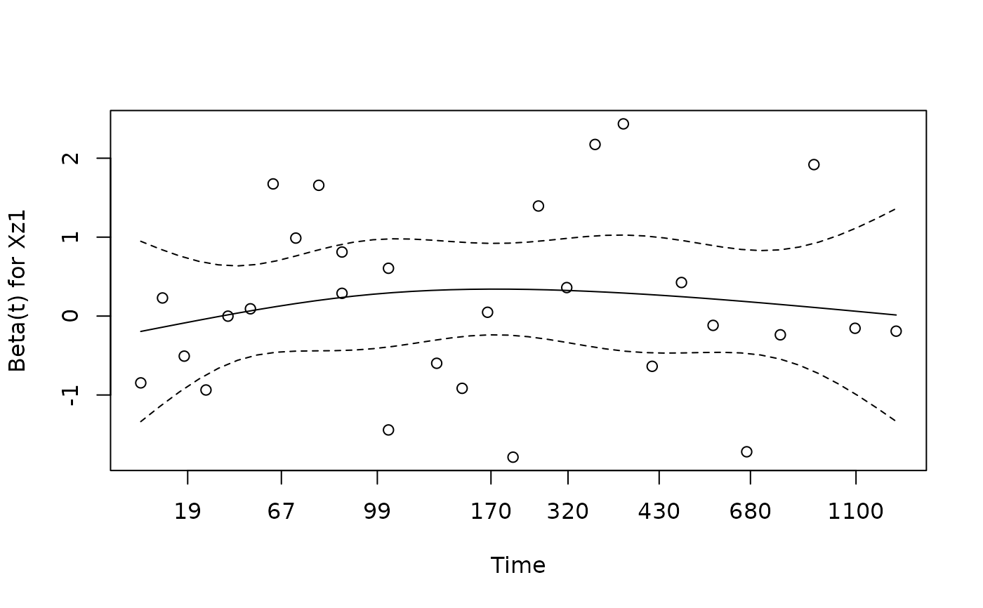
plot(fit$ph$ph11)
#> Warning: no non-missing arguments to min; returning Inf
#> Warning: no non-missing arguments to max; returning -Inf
#> Warning: no non-missing arguments to min; returning Inf
#> Warning: no non-missing arguments to max; returning -Inf
 #> Error in plot.window(...): need finite 'xlim' values
plot(fit$ph$ph10)
#> Warning: no non-missing arguments to min; returning Inf
#> Warning: no non-missing arguments to max; returning -Inf
#> Warning: no non-missing arguments to min; returning Inf
#> Warning: no non-missing arguments to max; returning -Inf
#> Error in plot.window(...): need finite 'xlim' values
#> Error in plot.window(...): need finite 'xlim' values
plot(fit$ph$ph10)
#> Warning: no non-missing arguments to min; returning Inf
#> Warning: no non-missing arguments to max; returning -Inf
#> Warning: no non-missing arguments to min; returning Inf
#> Warning: no non-missing arguments to max; returning -Inf
#> Error in plot.window(...): need finite 'xlim' values